Introduction to reinforcement learning and OpenAI Gym
A demonstration of basic reinforcement learning problems.
 Image from page 163 of "Mazes and labyrinths; a general account of their history and developments" (1922). (source: Internet Archive on Flickr)
Those interested in the world of machine learning are aware of the capabilities of reinforcement-learning-based AI. The past few years have seen many breakthroughs using reinforcement learning (RL). The company DeepMind combined deep learning with reinforcement learning to achieve above-human results on a multitude of Atari games and, in March 2016, defeated Go champion Le Sedol four games to one. Though RL is currently excelling in many game environments, it is a novel way to solve problems that require optimal decisions and efficiency, and will surely play a part in machine intelligence to come.
OpenAI was founded in late 2015 as a non-profit with a mission to “build safe artificial general intelligence (AGI) and ensure AGI’s benefits are as widely and evenly distributed as possible.” In addition to exploring many issues regarding AGI, one major contribution that OpenAI made to the machine learning world was developing both the Gym and Universe software platforms.
Gym is a collection of environments/problems designed for testing and developing reinforcement learning algorithms—it saves the user from having to create complicated environments. Gym is written in Python, and there are multiple environments such as robot simulations or Atari games. There is also an online leaderboard for people to compare results and code.
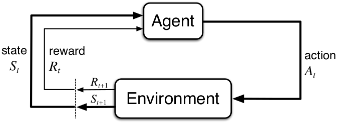
Reinforcement learning, explained simply, is a computational approach where an agent interacts with an environment by taking actions in which it tries to maximize an accumulated reward. Here is a simple graph, which I will be referring to often:

An agent in a current state (St) takes an action (At) to which the environment reacts and responds, returning a new state(St+1) and reward (Rt+1) to the agent. Given the updated state and reward, the agent chooses the next action, and the loop repeats until an environment is solved or terminated.
OpenAI’s Gym is based upon these fundamentals, so let’s install Gym and see how it relates to this loop. We’ll get started by installing Gym using Python and the Ubuntu terminal. (You can also use Mac following the instructions on Gym’s GitHub.)
sudo apt-get install -y python3-numpy python3-dev python3-pip cmake zlib1g-dev libjpeg-dev xvfb libav-tools xorg-dev python-opengl libboost-all-dev libsdl2-dev swig
cd ~
git clone https://github.com/openai/gym.git
cd gym
sudo pip3 install -e '.[all]'
Next, we can open Python3 in our terminal and import Gym.
python3
import gym
First, we need an environment. For our first example, we will load the very basic taxi environment.
env = gym.make("Taxi-v2")
To initialize the environment, we must reset it.
env.reset()
You will notice that resetting the environment will return an integer. This number will be our initial state. All possible states in this environment are represented by an integer ranging from 0 to 499. We can determine the total number of possible states using the following command:
env.observation_space.n
If you would like to visualize the current state, type the following:
env.render()
In this environment the yellow square represents the taxi, the (“|”) represents a wall, the blue letter represents the pick-up location, and the purple letter is the drop-off location. The taxi will turn green when it has a passenger aboard. While we see colors and shapes that represent the environment, the algorithm does not think like us and only understands a flattened state, in this case an integer.
So, now that we have our environment loaded and we know our current state, let’s explore the actions available to the agent.
env.action_space.n
This shows us there are a total of six actions available. Gym will not always tell you what these actions mean, but in this case, the six possible actions are: down (0), up (1), right (2), left (3), pick-up (4), and drop-off (5).
For learning’s sake, let’s override the current state to 114.
env.env.s = 114
env.render()
And, let’s move up.
env.step(1)
env.render()
You will notice that env.step(1) will return four variables.
(14, -1, False, {'prob': 1.0})
In the future we will define these variables as so:
state, reward, done, info = env.step(1)
These four variables are: the new state (St+1 = 14), reward (Rt+1 = -1), a boolean stating whether the environment is terminated or done, and extra info for debugging. Every Gym environment will return these same four variables after an action is taken, as they are the core variables of a reinforcement learning problem.
Take a look at the rendered environment. What do you expect the environment would return if you were to move left? It would, of course, give the exact same return as before. The environment always gives a -1 reward for each step in order for the agent to try and find the quickest solution possible. If you were measuring your total accumulated reward, constantly running into a wall would heavily penalize your final reward. The environment will also give a -10 reward every time you incorrectly pick up or drop off a passenger.
So, how can we solve the environment?
One surprising way you could solve this environment is to choose randomly among the six possible actions. The environment is considered solved when you successfully pick up a passenger and drop them off at their desired location. Upon doing this, you will receive a reward of 20 and done will equal True. The odds are small, but it’s still possible, and given enough random actions you will eventually luck out. A core part of evaluating any agent’s performance is to compare it to a completely random agent. In a Gym environment, you can choose a random action using env.action_space.sample(). You can create a loop that will do random actions until the environment is solved. We will put a counter in there to see how many steps it takes to solve the environment.
state = env.reset()
counter = 0
reward = None
while reward != 20:
    state, reward, done, info = env.step(env.action_space.sample())
    counter += 1

print(counter)
You may luck out and solve the environment fairly quickly, but on average, a completely random policy will solve this environment in about 2000+ steps, so in order to maximize our reward, we will have to have the algorithm remember its actions and their associated rewards. In this case, the algorithm’s memory is going to be a Q action value table.
To manage this Q table, we will use a NumPy array. The size of this table will be the number of states (500) by the number of possible actions (6).
import numpy as np
Q = np.zeros([env.observation_space.n, env.action_space.n])
Over multiple episodes of trying to solve the problem, we will be updating our Q values, slowly improving our algorithm’s efficiency and performance. We will also want to track our total accumulated reward for each episode, which we will define as G.
G = 0
Similar to most machine learning problems, we will need a learning rate as well. I will use my personal favorite of 0.618, also known as the mathematical constant phi.
alpha = 0.618
Next, we can implement a very basic Q learning algorithm.
for episode in range(1,1001):
    done = False
    G, reward = 0,0
    state = env.reset()
    while done != True:
            action = np.argmax(Q[state]) #1
            state2, reward, done, info = env.step(action) #2
            Q[state,action] += alpha * (reward + np.max(Q[state2]) - Q[state,action]) #3
            G += reward
            state = state2
    if episode % 50 == 0:
        print('Episode {} Total Reward: {}'.format(episode,G))
This code alone will solve the environment. There is a lot going on in this code, so I will try and break it down.
First (#1): The agent starts by choosing an action with the highest Q value for the current state using argmax. Argmax will return the index/action with the highest value for that state. Initially, our Q table will be all zeros. But, after every step, the Q values for state-action pairs will be updated.
Second (#2): The agent then takes action and we store the future state as state2 (St+1). This will allow the agent to compare the previous state to the new state.
Third (#3): We update the state-action pair (St , At) for Q using the reward, and the max Q value for state2 (St+1). This update is done using the action value formula (based upon the Bellman equation) and allows state-action pairs to be updated in a recursive fashion (based on future values). See Figure 2 for the value iteration update.

Following this update, we update our total reward G and update state (St) to be the previous state2 (St+1) so the loop can begin again and the next action can be decided.
After so many episodes, the algorithm will converge and determine the optimal action for every state using the Q table, ensuring the highest possible reward. We now consider the environment problem solved.
Now that we solved a very simple environment, let’s move on to the more complicated Atari environment—Ms. Pacman.
env = gym.make("MsPacman-v0")
state = env.reset()
You will notice that env.reset() returns a large array of numbers. To be specific, you can enter state.shape to show that our current state is represented by a 210x160x3 Tensor. This represents the height, length, and the three RGB color channels of the Atari game or, simply put, the pixels. As before, to visualize the environment you can enter:
env.render()
Also, as before, we can determine our possible actions by:
env.action_space.n
This will show that we have nine possible actions: integers 0-8. It’s important to remember that an agent should have no idea what these actions mean; its job is to learn which actions will optimize reward. But, for our sake, we can:
env.env.get_action_meanings()
This will show the nine possible actions the agent can chose from, represented as taking no action, and the eight possible positions of the joystick.
Using our previous strategy, let’s see how good a random agent can perform.
state = env.reset()
reward, info, done = None, None, None
while done != True:
    state, reward, done, info = env.step(env.action_space.sample())
    env.render()
This completely random policy will get a few hundred points, at best, and will never solve the first level.
Continuing on, we cannot use our basic Q table algorithm because there is a total of 33,600 pixels with three RGB values that can have a range from 0 to 255. It’s easy to see that things are getting extremely complicated; this is where deep learning comes to the rescue. Using techniques such as convolutional neural networks or a DQN, a machine learning library is able to take the complex high-dimensional array of pixels, make an abstract representation, and translate that representation into a optimal action.
In summary, you now have the basic knowledge to take Gym and start experimenting with other people’s algorithms or maybe even create your own. If you would like a copy of the code used in this OpenAI Gym tutorial to follow along with or edit, you can find the code on my GitHub.
The field of reinforcement learning is rapidly expanding with new and better methods for solving environments—at this time, the A3C method is one of the most popular. Reinforcement learning will more than likely play an important role in the future of AI and continues to produce very interesting results.
