Testing machine learning explanation techniques

Interpreting machine learning models is a pretty hot topic in data science circles right now. Machine learning models need to be interpretable to enable wider adoption of advanced predictive modeling techniques, to prevent socially discriminatory predictions, to protect against malicious hacking of decisioning systems, and simply because machine learning models affect our work and our lives. Like others in the applied machine learning field, my colleagues and I at H2O.ai have been developing machine learning interpretability software for the past 18 months or so.

We were able to give a summary of applied concerns in the interpretability field in an O’Reilly report earlier this year. What follows here are excerpts of that report, plus some new, bonus material. This post will focus on a few important, but seemingly less often discussed, interpretability issues: the approximate nature of machine learning interpretability techniques, and how to test model explanations.

Why do we need to test interpretability techniques?

Most serious data science practitioners understand machine learning could lead to more accurate models and eventually financial gains in highly competitive regulated industries…if only it were more explainable. So why isn’t everyone just trying interpretable machine learning? Simple answer: it’s fundamentally difficult, and in some ways, a very new field of research. Two of the toughest problems in machine learning interpretability are 1) the tendency of most popular types of machine learning models to combine and recombine input variables and 2) a phenomenon known as “the multiplicity of good models.” These two issues conspire to make nearly all machine learning interpretability techniques at least somewhat approximate.

Machine learning models combine variables, but we need explanations based on single variables

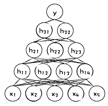
A primary mechanism by which popular machine learning models can generate more accurate predictions than more traditional linear models is by learning about high-degree interactions between input variables. Figure 1 presents a cartoon illustration of a simple artificial neural network (ANN). We can see that the original input variables, \(x_1-x_5\), are combined in the first hidden layer of the network, neurons \(h_{11}-h_{14}\), and recombined in the second hidden layer of the network, neurons \(h_{21}-h_{23}\), and recombined again in the third hidden layer of the network, neurons \(h_{31}\) and \(h_{32}\), before finally making a prediction.

While learning how to weigh complex combinations of input variables can lead to more accurate predictions, it makes explaining machine learning models really difficult. Most people, and some very serious regulatory statutes, prefer that decisions produced by predictive models be explained using the original input variables, not arbitrarily high-degree, scaled, weighted combinations of the input variables.

If you are rejected for a credit card, the lender doesn’t usually say it’s because the arctangent of a weighted, scaled combination of your debt-to-income ratio, your savings account balance, your ZIP code, your propensity to play tennis, your credit history length, and your credit score are equal to 0.57. Even though that may be how the model decided to reject you, lenders are typically required to break down the decision and attempt to explain it to you in simple terms, using one original input variable at a time and only the most important original input variables—for example, stating that your debt-to-income ratio is too high, that your credit score is too low, and your credit history is too short. For machine learning models, such disaggregation processes are often approximate and don’t really represent how machine learning models actually make predictions. This is a major reason why we should be using several different types of interpretability techniques to double check one another—and why we should test our machine learning interpretability techniques.

The multiplicity of good models

In his seminal 2001 paper, the UC Berkeley professor Leo Breiman popularized the phrase: “the multiplicity of good models.” The phrase means that for the same set of input variables and prediction targets, complex machine learning algorithms can produce multiple accurate models with very similar, but not the exact same, internal architectures. (Some in credit scoring refer to this phenomenon as “model locality.”)

Figure 2 is a cartoon depiction of a non-convex error surface that is representative of the error function for a machine learning algorithm with two inputs—say, a customer’s income and a customer’s interest rate—and an output, such as the same customer’s probability of defaulting on a loan. This non-convex error surface with no obvious global minimum implies there are many different ways a complex machine learning algorithm could learn to weigh a customer’s income and a customer’s interest rate to make a good decision about when they may default. Each of these different weightings would create a different function for making loan default decisions, and each of these different functions would have different explanations. All of this is an obstacle to interpretation because very similar predictions from very similar models can have different explanations. Because of this systematic instability, we should use several interpretability techniques to check explanations for a single model, we should seek consistent results across multiple modeling and interpretation techniques, and we should test our explanatory techniques.

How do we test interpretability techniques?

Since the approximate nature of machine learning explanations can, and often should, call into question the trustworthiness of model explanations themselves, we need to test explanations for accuracy. Don’t fret—it’s definitely possible! Originally, researchers proposed testing machine learning model explanations by their capacity to help humans identify modeling errors, find new facts, decrease sociological discrimination in model predictions, or to enable humans to correctly determine the outcome of a model prediction based on input data values. Human confirmation is probably the highest bar for machine learning interpretability, but recent research has highlighted potential concerns about pre-existing expectations, preferences toward simplicity, and other bias problems in human evaluation. Given that specialized human evaluation studies are likely impractical for most commercial data science or machine learning groups anyway, several other automated approaches for testing model explanations are proposed here (and probably other places too): we can use simulated data with known characteristics to test explanations; we can compare new explanations to older, trusted explanations for the same data set; and we can test explanations for stability. Using simulated data for testing explanations has been particularly fruitful for us at H2O, so we’ll dig into more details for that method in this post.

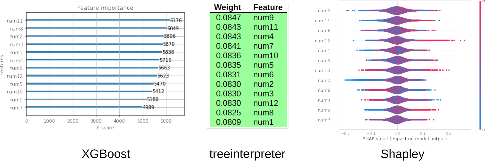
Models trained on totally random data with no relationship between a number of input variables and a prediction target should not give strong weight to any input variable nor generate compelling local explanations. Figure 3 displays the global variable importance, as calculated by three different tools: XGBoost, treeinterpreter, and shap, for an XGBoost GBM binary classification model trained on random data. From these three methods, which confirm one another, we can be fairly sure that the XGBoost model has not overfit the random signal to weigh any one variable over another, and we can see that the global explanations roughly match each other and the known situation in our simulated training data.

We can also test local variable importance in the same way. For the single row of data that represents the median prediction of the same XGBoost model trained on random data, we would expect that no one variable makes a large contribution to the model prediction and that these small local contributions were roughly randomly distributed between positive and negative contributions. Figure 4 shows us this result using the LIME, treeinterpreter, and shap methods, and should help bolster trust in both the model and the explanations. Now we see from a local perspective that XGBoost has not overfit the random data, that the explanatory tools roughly confirm one another, and that they match the known random signal in the training data.

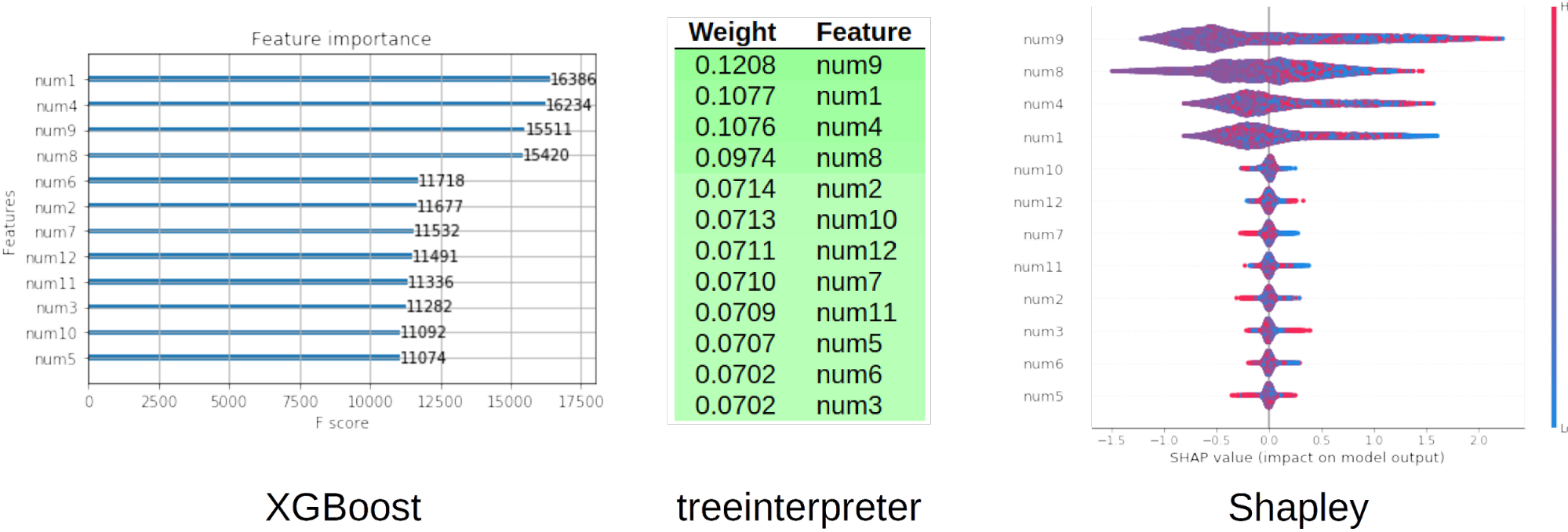
We can use simulated data with a known signal-generating function to test that explanations accurately represent that known function, too. Figure 5 shows the XGBoost, treeinterpreter, and shap global variable importance for an XGBoost GBM binary classifier model trained on the known signal-generating function, where \(e\) is a small random error term:

\(num1 * num4 +| num8 | * num9^2 + e\)

In Figure 5, we can see that although the three tools do not rank the important variables in exactly the same order, the model definitely learned that the four variables in the signal-generating function were more important than the other variables in our generated training data. The explanations portray the known ground truth in our simulated data experiment, which should increase our trust in both the modeling and explanatory methods.

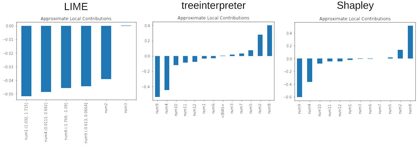
Figure 6 presents an example of local explanations using the same XGBoost model and simulated training data. Here we see something interesting. While all of the explanatory techniques see num9, num8, and num4 as important, they also pick up on the noise variable num2. If only one technique detected num2 as locally important, this would cast doubt on the validity of that explanatory technique. Since all three interpretability tools see num2 as locally important, it’s more likely that the model also sees num2 as important. This is an example of when interpretability techniques can help with model debugging.

Despite using a validation set and L1 and L2 regularization, our XGBoost model is learning that an unimportant variable, num2, is important around the median range of its predictions. Perhaps more training data, more validation data, cross-validation, more or different regularization, or other measures are needed to remedy this problem. The keys here are that the local interpretation techniques were necessary to spot this problem and all the local techniques agree that the model is giving num2 too much weight. Also, as expected for the median prediction, treeinterpreter and Shapley give roughly equal numbers of variables positive and negative local weights. However, LIME gives all important variables negative local weights. Has LIME failed in this case? Not likely. We have to remember that LIME explanations are usually offset from a local linear intercept. With a little digging, we can see the LIME model intercept was 0.7 for a GBM model prediction of 0.3. Given this information, it probably makes sense that LIME would see num1, num4, num8, and num9 as important but give them negative local weights.

We’ve shown several situations where explanations behave basically correctly, but we sometimes see explanations fail, and it’s much better to catch and debug those failures on simulated data than in production applications. Check out our h2oai/mli-resources GitHub repo

to see some of those failures, the details of some of the simulation tests we’ve discussed, and more examples of testing explanations using open source modeling and explanatory packages on simulated data.

Aside from testing against simulated data, we’ve toyed around with a few other programmatic methods for testing machine learning explanations that you might find helpful as well.

• Explanation stability with increased prediction accuracy

If previously known, accurate explanations from a simpler linear model are available, we can use them as a reference for the accuracy of explanations from a related, but more complex and hopefully more accurate, model. You can perform tests to see how accurate a model can become before its prediction’s explanations veer away from known standards.

• Explanation stability under data perturbation

Trustworthy explanations likely should not change drastically for minor changes in input data. You can set and test thresholds for allowable explanation value changes automatically by perturbing input data.

Conclusion

We’ll conclude with some important tips: test your explanatory tools, use more than one type of tool to explain your machine learning models, and look for consistent results across different explanatory methods. Moreover, remember that not all explanatory methods and tools are the same. Some are based on serious theory and are implemented with caution and rigor. Some are, well, not. From our experiences over the past 18 months, Shapley explanations really stand out as an excellent explanatory approach, especially when using tree-based modeling techniques. LIME seems to be the best option for other types of machine learning models, although it does have a few quirks. Shapley, LIME, and treeinterpreter—discussed in this post—are just a few of the many interpretability techniques available today. There are numerous other interpretability methods and tools with their own pros and cons, along with many types of interpretable models, and many fields and problem domains with their own interpretable machine learning needs. These topics and a lot more are covered in our longer report, so if this post was helpful, be sure to have a look there, too.